
Tech Corner
How will facial recognition systems & algorithms work in 2023?
Facial Recognition Systems first detect faces. They then get into feature extraction, next, they classify faces. Learn how these systems and algorithms work!
Time complexity is the amount of time that an algorithm takes to run as a function of the input. It is essentially the computational complexity that describes how much computer time it takes to run an algorithm.
It is generally estimated by counting the number of elementary operations that the algorithm performs, assuming that every elementary operation takes a fixed amount of time to perform. Therefore, the amount of time taken and the number of elementary operations performed by the algorithm is considered to differ by at most a constant factor.
Because an algorithm's running time could vary among different inputs of the same size, you would usually consider the worst-case time complexity. This is the maximum amount of time that is required for inputs of a particular size. The average case complexity is used less often, but is generally specified explicitly. This is the average time taken on inputs of a specific size. It makes sense since there is just a finite number of possible inputs of a given size.
In both situations, the time complexity tends to be expressed as a function of the size of the input. Because it is not easy to compute this function exactly, and the running time for small inputs tends to be inconsequential, you would generally concentrate on the behavior of the complexity as the input size increases. This is the asymptotic behavior of the complexity. Because of this, time complexity is generally expressed by making use of the big O notation, generally O(n), O(n log n), O(n), O(2n),etc. Here, n is the input size in bits that is needed to represent the input.
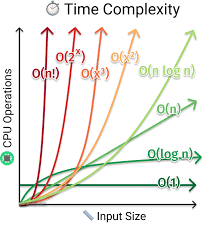
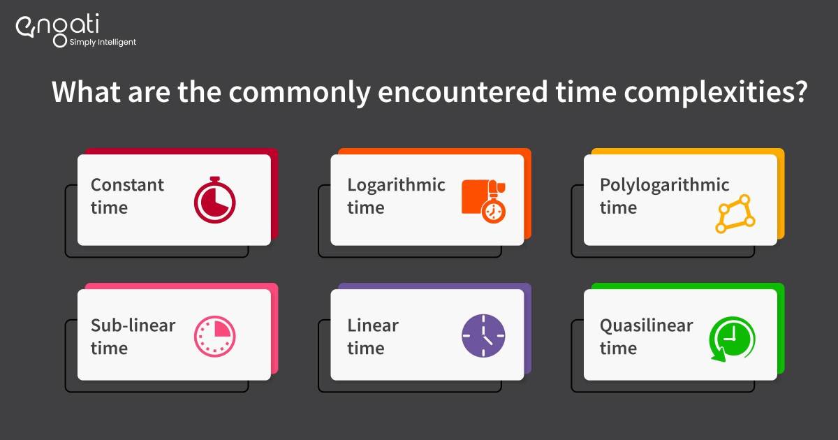
You can classify algorithmic complexities based on the type of function that appears in the big O notation.
Here are some of the common time complexities:
An algorithm is considered to be constant time, represented as O(1) time if the value of T(n) is bounded by a value that is independent of the size of the input. As an example, it takes constant time to access any single element in an array because just a single operation needs to be performed to locate it.
You can say that an algorithm takes logarithmic time if T(n) = O(log n). Because logan and logN are related by a constant multiplier and the multiplier has no relevance to big-O classification, the standard usage for logarithmic-time algorithms is O(log n) irrespective of the base of the logarithm appearing in the expression of T.
Logarithmic time is generally found in algorithms used in operations on binary trees and when using binary search.
You can say that an algorithm runs in polylogarithmic time if T(n) is O((log n)k) for a constant k. This could also be written as O(logkn).
As an example, you can solve matrix chain ordering in polylogarithmic time using a parallel random-access machine and you can determine a graph to be planar in a fully dynamic way in O(log3n) time for every insert/delete operation.
An algorithm runs on sublinear time if T(n) = o(n). This includes algorithms with the time complexities described earlier.
Sub-linear time algorithms are usually randomized and only provide approximate solutions. These algorithms arise naturally in the investigation of property testing.
An algorithm can be considered to take linear time if its time complexity is O(n). This means that the running time increases at the most in a linear manner as the size of the input increases. To explain this in a clearer fashion, there is a constant c such that the running time is cn at the most for each input whose size is n.
If the algorithm needs to sequentially read its entire input, then linear time is the best time complexity for those circumstances.
An algorithm running in quasilinear time (aka log-linear time) has T(n) = O(n logkn) for a positive constant k and linearithmic time is the case k = 1. Making use of the soft O notation, these algorithms are Õ(n). They are also O(n1+ε) for each constant ε that is greater than 0.
If an algorithm has T(n) = o(n2), then it runs on sub-quadratic time.
If an algorithm’s running time is upper bounded by a polynomial expression in the size of the input for the algorithm, i.e., (n) = O(nk) for a positive constant k, then it runs on polynomial time.
If T(n) isn’t upper bounded by a polynomial, the algorithm runs on superpolynomial time. Algorithms that use exponential resources are very obviously superpolynomial, but certain algorithms are just rather weakly superpolynomial.
These are algorithms that run longer than polynomial time but not long enough to be exponential time. Quasi-polynomial time algorithms generally arise in reductions from an NP-Hard problem to another problem.
This is when an algorithm can grow faster than any polynomial time, but is still far smaller than an exponential. Problems that have sub-exponential time are more tractable the problems that only have exponential algorithms.
If an algorithm has T(n) upper bounded by 2poly(n) and poly(n) is a polynomial in n, then it is in exponential time. The problems admitting exponential time algorithms on deterministic Turing machines belong to the complexity class known as EXP.
Bogosort is an example of an algorithm that runs on factorial time.
If T(n) is upper bounded 22poly(n), where poly(n) is a polynomial in n, then the algorithm runs in double exponential time. These algorithms are of the complexity class 2-EXPTIME.

Tech Corner
Facial Recognition Systems first detect faces. They then get into feature extraction, next, they classify faces. Learn how these systems and algorithms work!

Tech Corner
Looking for a cheatsheet to tune your Hyper-Parameters in Machine Learning and Neural Network Algorithms? We've got you covered! Click here to learn more.

Whatsapp Marketing
Learn how to create a WhatsApp bot in 5 minutes with easy steps. Discover WhatsApp integration tips, explore use cases & get a chatbot demo with free trail.